

Every college football season, there are teams who over- or under-perform on win totals due to inopportune turnovers, bad whistles, injuries or luck. Football is weird like that, and small samples can greatly influence seasonal outcomes.
Intuitively, we may expect teams that are extremely lucky (or unlucky) to regress positively or negatively to their “true” college football win total in the subsequent season. If we can identify these “outlier” teams, then we may stand to profit on that regression by betting their team win totals the following season.
That line of reasoning is fairly straightforward, but we have two hurdles to jump if we intend to craft a betting system based on it.
- How do we statistically define which teams qualify as “outliers?”
- Does historical win total data support the hypothesis that outlier teams experience win total regression in the following season?
Second-Order Wins
One method of identifying these outlier teams is to examine second-order (2ndO) win totals. In layman’s terms, a team’s 2ndO win total reports the cumulative win expectancy of each of its games throughout a season. I gleaned 2ndO wins from Football Outsiders, which offers a more comprehensive definition and statistical methods for deriving second-order wins.
Editor’s Note: Our NFL player prop packages are here. Get the early bird price and save — packages starting at just $49.95 for the full season.
For this study, we’re particularly interested in teams’ second-order win differential, which is the difference between a team’s actual wins and its 2ndO wins. Basically, how many games should this team have won based on its statistical performance?
For example, Ohio State went 13-1 last season but only managed 10.9 2ndO wins. So, the Buckeyes over-performed expectation by 2.1 wins.
On the flip-side of the same coin, UTEP managed just a single win in 2018, but the Miners had 3.2 second-order wins. That yields a differential of +2.2 wins and suggests Miner Nation may have cause for optimism in 2019.
The big thing to keep in mind here is that a negative 2ndO win differential suggests that a team over-performed in the previous season, and a positive 2ndO win differential suggests that a team under-performed.
Analyzing Historical College Football Win Data
The source population of team win totals since 2006 is 1,731, so the provided sample constitutes 28.8% of our target population.

It would be ideal if I could find a full inventory of win totals since 2006, but a sample size of 499 is still significant. Admittedly, it’s small enough to potentially be skewed, especially since most of the teams in the sample are very public teams (Alabama, Clemson, USC, Notre Dame, etc.) rather than, say, UTSA or Western Kentucky. However, I still feel confident the sample is large enough to render statistically significant descriptive results.
With that disclaimer out of the way, let’s dive into my methods and results. I recorded previous-season 2ndO win differentials for every team in our sample. Then, I evaluated whether or not 2ndO win differential had a meaningful effect on teams going over or under their next-season win total.
Results
I broke up our sample into two groups:
- Teams who over-performed their win total (-3.3 to -0.1)
- And those who under-performed (+0.1 to +3.3) in the previous season
Over-performers report a healthy 135-111-26 under record (54.9%) for their team win totals in the following season. However, under-performers do not rebound quite as much as expected, reporting an over record of just 92-86-25. Altogether, the under hits 52.0% of the time across all teams, which may suggest that the public is biased towards betting overs.
Next, let’s visualize our data set in terms of net units won or lost by 2ndO win differential:
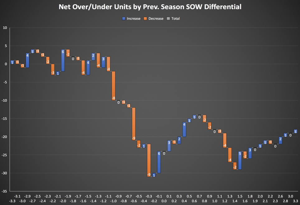
The above graph paints a significantly different picture than our basic summary statistics. This visualization reinforces the overall under trend, but it also reveals a small over trend in the upper part of the tail (teams with a 2ndO differential of +1.5 or higher).
Conveniently, the over trend in the upper tail represents “outlier” teams who under-performed in the previous season, which supports our original hypothesis regarding regression to the mean.
However, while this chart is easy to understand visually, it does have a flaw: It reports net units won or lost — not betting volume or win-rate. So, let’s break down each of the major trends in the above graph in terms of total over-under record and sample size.
Betting Win Totals on Extreme Under-Performers
The +1.5 to +3.3 range in the upper tail of our graph offers huge value on the over (69.0% over-rate), but it suffers from a tiny sample size (35). If you expand this range to include the larger over trend beginning at -0.2, the over reports a 122-109-29 record (52.8% hit-rate). That larger trend still favors the over, but only marginally so.
Nonetheless, the rarity of teams at the extreme upper end of the distribution — combined with the exorbitant over-rate of 69.0% — should pique your interest. While this particular over trend likely isn’t strong enough to stand alone due to sample size issues, it could serve as reinforcement in your decision to take the over on such teams if the trend matches your intuition or primary research analysis.
Betting Win Totals on Extreme Over-Performers
At the bottom tail of our distribution (-3.3 to -1.2), bettors largely get chewed up with no discernible trend. Against intuition, teams in this range do not rebound strongly in the following season. Perhaps this indicates that their regression is largely priced into their preseason win totals. Regardless, it’s best to tread with caution for teams in this range.
Strong Under Trends for the Middle of The Distribution
In the middle of our distribution, we’ve got some interesting things going on:
- There are two strong under trends from -1.1 to -0.3 and from +0.8 to +1.4
- Oddly, interposed between those trends is a moderate over trend from -0.2 to +0.7
However, if you analyze the entire range from -1.1 to +1.4, the under hits 54.5% of the time with a total record of 187-156-37. Most importantly, this range has a sample size of 380-of-499 teams, which adds significant statistical weight to this trend compared to others analyzed herein.
How to Play It
The under reports a 232-214-53 for the entire dataset, which suggests that the under is the preferred position if you’re betting blind. Moreover, by excluding the over trend in the upper tail and the chewed-up noise in the lower tail, you can more tightly focus your under plays on these teams in the middle.
Teams with a previous season 2ndO win differential of -1.1 to -0.3 go under their preseason win total at a 61.7% clip (87-54-14 overall) with a healthy sample size of 155. If you’re going to target any particular range of teams, this is likely the range to do it.
However, be advised that there’s no intuitive rationale explaining why teams in this range tend towards the under. They don’t exist at the fringe of our distribution, and so they don’t match our original hypothesis. Be cautious in betting any trend like this blindly without consulting secondary research to justify your position.
2019 Teams That Fit Our Over Trend
The following teams fit our over trend with a 2018-19 second-order win differential of +1.5 to +3.3 (2ndO differential in parentheses):
- Texas State (+3.1)
- Nebraska (+2.7)
- UTEP (+2.2)
- USC (+2.0)
- Miami (FL) (+1.8)
- North Carolina (+1.8)
- Florida Atlantic (+1.6)
- Memphis (+1.6)
- Eastern Michigan (+1.5)
- Purdue (+1.5)
Among these teams, three stand out as strong potential over bets: Miami(FL), Memphis, and North Carolina.
- Memphis – 9.5 (-125o)
- Miami (FL) – 8.5 (-135o)
- North Carolina – 4.5 (-165o)
Later this week, I’ll be publishing a follow-up piece to break down why I think these three particular teams are deserving of a potential over bet this season.
2019 Teams That Fit Our Under Trend
The following teams fit our under trend with a 2018-19 second-order win differential of -1.1 to -0.3 (2ndO differential in parentheses).
- Akron (-1.1)
- Boise State (-1.1)
- Clemson (-1.0)
- Utah State (-1.0)
- Louisiana Tech (-0.9)
- LSU (-0.9)
- UAB (-0.9)
- Ball State (-0.9)
- Boston College (-0.8)
- Hawai’i (-0.8)
- Arizona State (-0.7)
- Tennessee (-0.7)
- NC State (-0.7)
- Bowling Green (-0.6)
- Connecticut (-0.6)
- Florida State (-0.6)
- Northern Illinois (-0.6)
- Stanford (-0.6)
- Louisiana-Monroe (-0.6)
- Western Michigan (-0.6)
- Buffalo (-0.5)
- California (-0.5)
- Rice (-0.5)
- West Virginia (-0.5)
- Tulane (-0.4)
- New Mexico State (-0.4)
- Florida (-0.3)
- Oklahoma (-0.3)
- Louisville (-0.3)
- Indiana (-0.3)
- South Florida (-0.3)
- Virginia Tech (-0.3)
Some of these teams make more sense than others. For example, I’m not touching Clemson’s consensus 11.5 win total, despite their inclusion in the list above. Nonetheless, the combination of this group’s strong under-rate and relatively large sample size should serve as encouragement to wager an under bet against any of them — provided that you have secondary research to support that position.
Also of particular note, NC State and West Virginia both make this list of potential under bets, and those two teams face each other in Week 3. After reviewing both of their team profiles, schedules, and projected S&P+, I don’t believe it’s worthwhile to lock up money on either team’s under for the full season. If you’re particularly interested in an under bet on either NC State or West Virginia, consider taking a side in their Week 3 matchup instead.